


























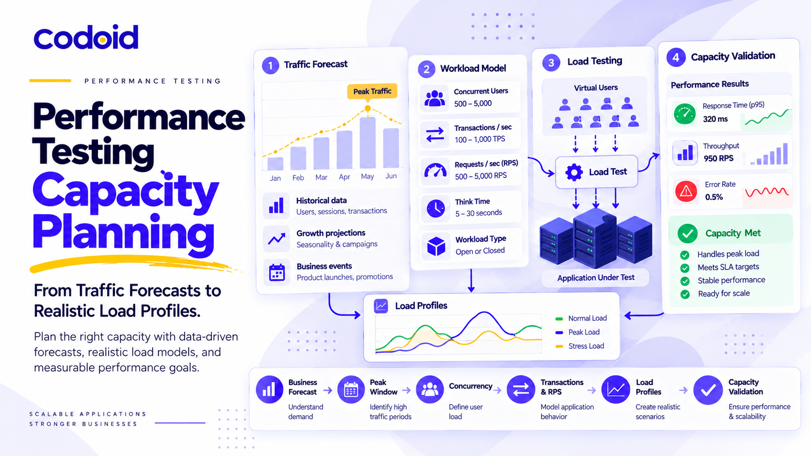
Performance testing often fails before a single request is sent. The test runs successfully, the dashboards turn green, and the report says the system handled the load. Then production traffic arrives at a different shape, and the application that passed the test starts dropping requests, exhausting connection pools, or losing capacity as response times climb. The gap usually sits in the workload model. A test configured for 20,000 concurrent threads is not the same as a test configured for the traffic profile the business actually expects. Performance Testing Capacity Planning closes that gap by translating a business forecast into a technically measurable workload with traceable assumptions. This guide walks through that conversion step by step. It starts with a business forecast, derives peak-window traffic, calculates concurrent users, translates sessions into business transactions, maps those transactions to requests per second, and builds a set of load profiles that validate the system against realistic demand. Codoid’s performance testing services apply this same conversion discipline to production capacity engagements.
Related Blogs
Cloud Performance Testing with Apache JMeter: A Practical Guide
Top Performance Testing Tools: Essential Features & Benefits.
- Direct Answer
- What Is Performance Testing Capacity Planning?
- Why Does Accurate Workload Modeling Matter?
- Concurrent Users vs Virtual Users vs RPS vs In-Flight Requests
- How Does Business Traffic Become a Technical Load Model?
- Step 1: Define the Business Forecast Precisely
- Step 2: Convert Long-Range Forecasts Into Peak Traffic
- Step 3: Convert Sessions per Hour Into Concurrent Users
- Step 4: Convert Business Sessions Into Transactions per Second
- Step 5: Convert Business Transactions Into Requests per Second
- Step 6: Account for Think Time and Pacing
- Step 7: Decide Whether the Workload Should Be Open or Closed
- Step 8: Size Virtual Users for an Arrival-Rate Test
- Step 9: Calculate In-Flight Request Concurrency
- Practical Example: Converting an E-Commerce Forecast
- Building the Load Profile
- What Should Be Measured During the Test?
- Best Practices for Performance Testing Capacity Planning
- Common Capacity-Planning Mistakes
- Troubleshooting Capacity Calculations
- Tools for Implementing Capacity-Based Load Tests
- Limitations and Risks of Capacity Calculations
- Conclusion
Direct Answer: How Do You Convert a Traffic Forecast Into a Performance-Test Workload?
To convert a business traffic forecast into a performance-testing capacity model, first express the forecast in a meaningful peak time window, such as sessions per peak hour or transactions per minute. Then calculate concurrent active users from session arrival rate and session duration, translate business journeys into requests per second (RPS) using the number and mix of backend requests each journey generates, and finally construct a load profile that reproduces normal, peak, spike, sustained, and failure-boundary traffic.
The fundamental relationships are:
    Concurrent Users = (Sessions in peak window × Average session duration)
                       ÷ Peak window duration

    For an hourly forecast:

    Concurrent Users = (Sessions per hour × Session duration in seconds) ÷ 3600
Grafana’s k6 documentation recommends this same relationship when converting hourly session analytics into concurrent-user estimates.
Aggregate RPS is calculated as:
RPS = Total requests ÷ Seconds
For systems with multiple user journeys:
    Total RPS = Σ (Journey Starts/sec_i × Requests/journey_i)
                i=1 to n
Do not assume that one concurrent user equals one request per second. Users spend time reading, typing, navigating, and waiting, while one business action can generate multiple HTTP requests.
Key Takeaways
- Start with peak-window traffic, not monthly or daily averages.
- Treat active users, virtual users, transactions, RPS, and in-flight requests as separate metrics.
- Calculate concurrency from the arrival rate and the time users remain active.
- Calculate RPS from the number of business actions and the request fan-out generated by those actions.
- Use open workload models when maintaining a specified transaction or request arrival rate matters. Use closed models when reproducing a finite population of active users matters.
- Build multiple load profiles, including expected peak, headroom, spike, soak, and breakpoint, instead of relying on one arbitrary VU count.
What Is Performance Testing Capacity Planning?
Performance testing capacity planning is the process of translating expected business demand into a technically measurable workload that can be generated against an application.
Its purpose is to answer questions such as:
- How many users may be active simultaneously?
- How many business transactions must the platform complete per second?
- How many HTTP or RPC requests will reach each service?
- How quickly will traffic rise?
- How long will peak traffic last?
- What happens if demand exceeds the forecast?
- Does autoscaling add capacity quickly enough?
- At what workload do latency, errors, queues, or resource utilization become unacceptable?
Performance testing capacity planning therefore sits between business forecasting and technical capacity validation.
Google’s SRE guidance describes capacity planning as combining organic demand growth with inorganic events such as launches or campaigns, then using regular load testing to correlate infrastructure capacity with actual service capacity.
It is different from infrastructure capacity planning alone. An infrastructure plan might say, “We expect 40 application instances.” A performance capacity model asks, “What business workload must those 40 instances successfully serve while meeting the required latency, availability, and error-rate objectives?”
Why Does Accurate Workload Modeling Matter?
A performance test can execute successfully while testing the wrong workload.
For example, suppose a retailer expects 20,000 concurrent customer sessions during a sale. A test configured for 20,000 threads that execute requests continuously with no realistic pacing could generate several times the actual production RPS.
The opposite problem is equally dangerous. A closed-user test may begin with the correct number of users, but as server response times increase, each user completes fewer iterations. The generated transaction rate therefore falls precisely when the application becomes overloaded. Grafana describes this behavior as a drawback of closed workload models and associates it with the coordinated-omission problem.
Google SRE similarly recommends establishing capacity through testing rather than assuming historical server-to-throughput relationships remain unchanged, because application changes can alter how much traffic the same infrastructure can process.
Accurate workload modeling is therefore necessary for both sides of capacity planning:
- Demand: What load will customers and integrations create?
- Supply: How much of that load can the current architecture process while satisfying its SLOs?
Concurrent Users vs Virtual Users vs RPS vs In-Flight Requests
These terms are related but are not interchangeable. Distinguishing them is central to accurate performance testing capacity planning.
| S. No | Metric | What it represents | Typical calculation | Best use |
|---|---|---|---|---|
| 1 | Concurrent active users | Real users or sessions active during the same period | Sessions × average duration ÷ observation window | Business workload sizing |
| 2 | Virtual users (VUs) | Execution workers representing simulated users in a test tool | Depends on workload model and scenario duration | Load-generator configuration |
| 3 | Transactions/sec | Completed or initiated business operations per second | Transactions ÷ seconds | Business-service capacity |
| 4 | Requests/sec (RPS) | HTTP or RPC requests arriving each second | Requests ÷ seconds | API and service capacity |
| 5 | In-flight requests | Requests currently being processed or waiting | RPS × average time in system | Connections, threads, queues, service concurrency |
| 6 | Throughput | Work processed per unit of time | Completed operations ÷ time | Capacity measurement |
Apache JMeter defines throughput as requests divided by elapsed time, while its thread groups use independent threads to simulate concurrent activity.
The distinction becomes important because a user may remain active for several minutes while issuing requests only intermittently.
A system can therefore have 15,000 concurrent customer sessions, 1,800 HTTP requests per second, and 400 requests actively in flight at approximately the same moment. Those numbers are not contradictory. They measure different layers of the workload.
How Does Business Traffic Become a Technical Load Model?
A reliable conversion follows this flow:
    Business forecast
        ↓
    Peak time window
        ↓
    User and session arrival rate
        ↓
    Concurrent active sessions
        ↓
    Business journey mix
        ↓
    Transaction arrival rates
        ↓
    Request fan-out
        ↓
    Endpoint and service RPS
        ↓
    Load profile
        ↓
    Performance and capacity validation
Each transformation should be documented so that someone can trace a performance-test target back to the original business assumption.
Step 1: Define the Business Forecast Precisely
Avoid starting with numbers such as “We expect 5 million users.” That number does not describe a load.
Instead, establish the forecast’s dimensions:
- Population: Sessions, customers, devices, API consumers, orders, or events?
- Window: Month, day, peak hour, five-minute peak, or one-minute spike?
- Region: Global or per deployment region?
- Channel: Web, mobile, partner API, batch, internal integration?
- Growth source: Organic adoption, campaign, product launch, seasonal event, migration?
- Traffic mix: Browse, search, login, checkout, upload, reporting, API integrations, and so on?
A useful requirement looks more like this: the EU deployment is forecast to receive 120,000 customer sessions during the busiest hour of the launch, with an average active session duration of six minutes.
That statement can be converted into concurrency.
Step 2: Convert Long-Range Forecasts Into Peak Traffic
Suppose the business forecasts 2.4 million sessions per day.
Dividing by 24 and testing 100,000 sessions per hour assumes traffic is evenly distributed throughout the day. Production traffic rarely behaves that way.
Instead, determine the actual or predicted fraction occurring in the peak interval:
Peak Sessions/hour = Daily Sessions × Peak Hour Fraction
If 14% of the daily sessions historically arrive during the busiest hour:
2,400,000 × 0.14 = 336,000 sessions/hour
The 14% value must come from analytics, monitoring, or a documented forecast assumption. It should not be invented simply to create a load test.
Grafana’s concurrent-user guidance explicitly recommends hourly rather than daily or monthly views because broad averages can hide important intraday traffic peaks.
Forecasts should also account separately for unusual demand sources. Google SRE distinguishes organic growth from inorganic demand created by events such as marketing campaigns or feature launches.
Step 3: Convert Sessions per Hour Into Concurrent Users
Assume the following:
- Peak sessions = 120,000 per hour
- Average active session duration = 6 minutes
- Six minutes = 360 seconds
Then:
    Concurrent Users = (120,000 × 360) ÷ 3600

    Concurrent Users = 12,000
The expected business peak therefore represents approximately 12,000 concurrently active sessions.
This is an application of the same arrival-rate and time relationship represented by Little’s Law:
L = λW
where the average number present in a stable system equals the arrival rate multiplied by average time spent in that system.
Important Limitation
The result is an average concurrency within the selected period.
It does not prove that concurrency will never exceed 12,000. Session arrivals and session durations have distributions, and short bursts can produce higher instantaneous concurrency.
Use high-resolution production telemetry when short-duration peaks matter.
Step 4: Convert Business Sessions Into Transactions per Second
Users do not generate HTTP requests merely by remaining logged in. They perform business actions.
Suppose analytics show that an average session produces:
- 5 product searches
- 12 product-detail views
- 2 cart updates
- 0.4 checkout attempts
- 0.2 account updates
The peak-hour business transaction rate for product searches becomes:
    Searches/sec = (120,000 × 5) ÷ 3600

    Searches/sec = 166.7
Product-detail transactions become:
    Product views/sec = (120,000 × 12) ÷ 3600

    Product views/sec = 400
Perform the same calculation for every significant workflow.
This gives the application team a business workload model, which is usually much more meaningful than simply selecting a number of test-tool threads.
Step 5: Convert Business Transactions Into Requests per Second
A business transaction is not necessarily one HTTP request.
A search operation may call an API gateway, a search service, a recommendation service, a pricing service, and an inventory service. Some calls may happen synchronously. Others may execute in parallel or asynchronously.
For workload (i):
RPS_i = Journey Starts/sec_i × Requests/Journey_i
Across all workloads:
    Total RPS = Σ (Journey Starts/sec_i × Requests/journey_i)
                i=1 to n
For a specific downstream endpoint (j):
    Endpoint RPS_j = Σ (Journey Starts/sec_i × Calls_i,j)
                      i=1 to n
This service-level calculation is often more valuable than total edge RPS because two workloads with identical edge throughput can put radically different pressure on databases, caches, queues, and downstream services.
Google’s launch guidance specifically warns that one page view can translate into many requests and recommends validating request-volume assumptions.
Step 6: Account for Think Time and Pacing
Real users pause. They read product descriptions, enter data, compare results, authenticate, switch screens, and occasionally abandon their sessions.
If a test omits those pauses, the VUs will execute workflows as rapidly as the application can respond.
For a closed-user model:
    Approximate RPS = (VUs × Requests per journey)
                      ÷ Average Iteration Duration
The iteration duration should include realistic user pacing where the objective is to model humans.
Consider the following:
- 10,000 VUs
- 8 requests per journey
- Average journey duration including think time = 80 seconds
Then:
RPS = (10,000 × 8) ÷ 80 = 1,000
Removing 40 seconds of think time would approximately double the resulting throughput even though the VU count remains unchanged.
Locust, for example, exposes wait-time and constant-pacing mechanisms specifically for controlling the time between simulated user tasks.
Related Blogs
JMeter Tutorial: An End-to-End Guide
JMeter vs Gatling vs k6: Comparing Top Performance Testing Tools
Step 7: Decide Whether the Workload Should Be Open or Closed
This is one of the most important choices in capacity-oriented performance testing capacity planning.
Closed Workload Model
A fixed population of VUs repeatedly executes a workflow. A VU finishes an iteration before beginning its next iteration.
This model works well when the requirement is naturally expressed as: simulate 10,000 users concurrently using the application.
The risk is that throughput depends on response time. If the application becomes slower, each VU takes longer to finish its journey, so transaction arrivals can decline.
Open Workload Model
Transactions or iterations start according to an external arrival schedule rather than waiting for previous iterations to finish.
This model is appropriate when the requirement is: the service must receive 2,000 checkout operations per second even if response time increases.
Grafana k6 implements open workloads through its arrival-rate executors and explains that the approach decouples new iteration starts from the system’s response time.
Practical Rule
- Use a closed model when concurrency is the contractual workload.
- Use an open model when arrival rate or throughput is the contractual workload.
- A mature test program may need both.
Step 8: Size Virtual Users for an Arrival-Rate Test
Even an open workload generator needs enough execution workers to sustain the desired arrival rate.
A useful first approximation is:
Required VUs = Iteration Arrival Rate × Iteration Duration
Suppose the target is 250 journey starts per second and average journey execution time is 4 seconds. Then:
Required VUs = 250 × 4 = 1,000
The test should normally allocate additional capacity for iteration-duration variability and degradation under load.
Grafana k6 documents a similar planning relationship for arrival-rate tests and recommends pre-allocating sufficient VUs. If too few are available, scheduled iterations can be dropped.
Do not treat the first calculation as a hard capacity number. Run a calibration test and observe actual iteration-duration distributions and load-generator resource usage.
Step 9: Calculate In-Flight Request Concurrency
User concurrency is different from server-side request concurrency.
For a stable service:
Average In-Flight Requests = RPS × Average Response Time
If an API receives 2,000 RPS and average response time is 200 ms:
In-Flight = 2,000 × 0.2 = 400
This helps reason about connection pools, worker threads, queue depth, database connections, downstream concurrency, and memory associated with active requests.
Microsoft’s Azure Load Testing documentation describes the inverse relationship for a simple case. Required VUs can be estimated as RPS multiplied by application latency.
That approximation is most directly applicable when VUs continuously issue requests. User journeys containing think time or multiple requests require a fuller workload model.
Practical Example: Converting an E-Commerce Forecast Into a Load Test
Consider a fictional e-commerce platform preparing for a product launch. The business forecast is:
| S. No | Input | Forecast |
|---|---|---|
| 1 | Peak sessions | 120,000 per hour |
| 2 | Average session duration | 6 minutes |
| 3 | First-party backend requests | 42 requests per session |
| 4 | Additional certification headroom | 25% |
The 42 requests per session are assumed to have been measured from representative production telemetry after removing static CDN traffic and unapproved third-party services.
Calculate Expected Concurrent Users
(120,000 × 360) ÷ 3600 = 12,000
Expected peak concurrency is 12,000 active sessions.
With the separately documented 25% certification margin:
12,000 × 1.25 = 15,000
Certification target is 15,000 concurrent sessions.
Calculate Expected Aggregate RPS
(120,000 × 42) ÷ 3600 = 1,400
Expected peak backend traffic is 1,400 RPS.
Certification target:
1,400 × 1.25 = 1,750 RPS
Service Group Breakdown
| S. No | Service group | Calls per session | Expected RPS | RPS with 25% headroom |
|---|---|---|---|---|
| 1 | Catalog and product | 14 | 466.7 | 583.3 |
| 2 | Search | 8 | 266.7 | 333.3 |
| 3 | Recommendations | 6 | 200.0 | 250.0 |
| 4 | Cart | 5 | 166.7 | 208.3 |
| 5 | Authentication and account | 3 | 100.0 | 125.0 |
| 6 | Checkout orchestration | 2 | 66.7 | 83.3 |
| 7 | Other first-party APIs | 4 | 133.3 | 166.7 |
| 8 | Total | 42 | 1,400 | 1,750 |
This table is already more useful to architecture teams than “15,000 users” because it identifies where the forecasted load actually lands.
Building the Load Profile
A capacity plan should not become a single flat test.
For the example above, a test suite could contain the following profiles:
| S. No | Profile | Illustrative workload | Purpose |
|---|---|---|---|
| 1 | Smoke | Small representative traffic | Validate script and test data |
| 2 | Baseline | Current production-like traffic | Establish comparison baseline |
| 3 | Forecast peak | Ramp to 1,400 RPS and hold | Validate expected launch traffic |
| 4 | Certification and headroom | Hold 1,750 RPS | Validate documented planning margin |
| 5 | Spike | Rapid transition above expected peak | Validate burst handling and recovery |
| 6 | Soak | Sustained representative high load | Detect leaks, queue growth, exhaustion, and degradation |
| 7 | Breakpoint | Gradually increase until a defined threshold fails | Discover usable capacity boundary |
The exact multipliers and durations should come from business risk, autoscaling characteristics, historical burst behavior, SLOs, and recovery objectives rather than an industry-wide arbitrary percentage.
Google SRE recommends testing both gradual and sudden load changes because caching and other system behavior can make the results different.
AWS similarly recommends covering average usage, peak loads, rapid spikes, and sustained high loads when testing scalability and performance.
What Should Be Measured During the Test?
Capacity is not simply the highest RPS reached before the application crashes. A usable capacity boundary should be defined against the service’s requirements.
Measure at least the following categories.
Client-Side
- Achieved arrival rate
- Achieved RPS and TPS
- Response-time percentiles
- Error rate
- Timeouts
- Connection errors
- Dropped or missed iterations
Application
- Request latency by endpoint
- Request count
- Error rate
- Queue depth
- Thread and worker utilization
- Connection-pool utilization
- Garbage-collection behavior
- Cache hit and miss rate
Infrastructure
- CPU
- Memory
- Network
- Disk and storage latency
- Pod or instance count
- Autoscaling activity
- Service quotas
Dependencies
- Database query latency
- Connection utilization
- Message-broker lag
- Downstream service latency
- Retry volume
- Rate limiting
Google SRE’s capacity model explicitly links demand, capacity, and software efficiency, emphasizing that a slowing service effectively loses capacity as load rises.
Best Practices for Performance Testing Capacity Planning
Derive the Workload From Production Evidence
Use analytics, access logs, distributed traces, APM telemetry, queue metrics, and business transaction data. Forecasting should extend observed behavior rather than replacing it with assumptions.
Preserve the Business-to-Technical Calculation
Store the forecast, conversion formulas, scenario distribution, request fan-out, and safety-margin assumptions alongside the performance-test configuration. A target such as “2,000 RPS” should always be explainable.
Model Each Significant User Population Separately
Web customers, mobile users, partner APIs, batch integrations, administrative traffic, and asynchronous workers frequently have different traffic patterns. Combining everything into one average workload can hide the service that actually becomes saturated.
Separate Edge Traffic From Internal Amplification
One incoming API request may trigger several RPCs, database operations, queue messages, or retries. Capacity-plan the important internal layers as well as the public endpoint. Codoid’s REST API testing checklist covers validation techniques for the endpoint layer that feeds these downstream calls.
Use Distributions Instead of Identical Think Times
Thousands of users pausing for exactly five seconds can unintentionally synchronize traffic. Randomized or production-derived pacing generally creates a more representative arrival pattern.
Use Production-Like Data and Cache Behavior
A test where every user repeatedly reads the same product can create unrealistically high cache hit rates. Conversely, forcing every request to be unique may create unrealistically low cache effectiveness.
Keep Third-Party Systems Outside the Test Unless Authorized
Browser journeys can call payment services, analytics systems, identity providers, social platforms, and other external endpoints. Grafana’s website load-testing guidance recommends excluding third-party requests unless permission exists to load test those systems.
Validate the Load Generator
A performance test measures the application correctly only when the generator itself can maintain the target workload. Apache JMeter recommends considering generator hardware, thread count, test-plan design, and distributed execution for large workloads.
Test Realistic Infrastructure
AWS recommends using an environment that closely mirrors production because scaled-down environments can produce inaccurate predictions of production behavior.
Common Capacity-Planning Mistakes
| S. No | Mistake | Why it happens | Impact | Recommended fix |
|---|---|---|---|---|
| 1 | Using monthly users as VUs | Business and test terminology are confused | Arbitrary load | Convert to sessions and peak-window arrivals first |
| 2 | Dividing daily traffic evenly by 24 | Peak distribution is unavailable | Peak load is underestimated | Use hourly or minute analytics |
| 3 | Assuming 1 user equals 1 RPS | Concurrency and throughput are conflated | Incorrect capacity target | Measure actions and requests per session |
| 4 | Treating one business transaction as one request | Internal request fan-out is ignored | Backend services are undertested | Map journeys to endpoint calls |
| 5 | Ignoring think time | Scripts execute as fast as possible | Generated RPS exceeds production | Add production-derived pacing |
| 6 | Skipping the load-generator validation | Focus is entirely on the target | Generator becomes the bottleneck | Measure generator CPU, memory, and network |
Troubleshooting Capacity Calculations
Why does the test produce less RPS than expected?
Review the scenario itself before suspecting the application. Common causes include:
- Requests per iteration
- Think time
- Parallel requests
- Automatic retries
- Redirects
- Polling
- Static-resource traffic
- Background requests
The test may have the correct VU count but the wrong user behavior. Calculate RPS from the script itself and compare it with production traces.
Why does the same total RPS produce different infrastructure utilization?
RPS alone does not describe workload cost.
A read-heavy request served from cache may consume very little compute, while a write operation involving validation, database updates, cache invalidation, events, and downstream services can consume much more.
Compare transaction mix, payload sizes, database queries, cache hit rate, retry volume, and internal service fan-out.
Why does an arrival-rate test report dropped iterations?
One possible cause is insufficient VUs available to begin the scheduled work. Grafana k6’s arrival-rate documentation explains that when the allocated VU pool cannot sustain the requested iteration rate, the tool records dropped iterations. Longer iteration durations require more available VUs.
Also inspect the load generator itself. CPU, memory, network bandwidth, TLS processing, or connection limits can prevent the generator from producing the intended load.
Why does a test environment pass while production struggles?
Compare the environments for differences in instance types, topology, scaling limits, service quotas, network routes, database size, cache state, data distribution, dependency behavior, feature flags, and security layers.
AWS recommends production-like environments specifically because reduced environments can lead to inaccurate predictions of production scaling behavior.
Tools for Implementing Capacity-Based Load Tests
| S. No | Tool or platform | Workload-model capabilities | Useful capacity-planning application |
|---|---|---|---|
| 1 | Grafana k6 | VU-based and arrival-rate executors | Explicit VU or transaction-arrival modeling |
| 2 | Apache JMeter | Thread groups, timers, throughput controls, experimental Open Model Thread Group | User concurrency and throughput-driven workloads |
| 3 | Locust | User classes, wait-time and pacing controls, custom load shapes | Code-driven user behavior and flexible traffic shapes |
| 4 | Azure Load Testing | VU- and RPS-oriented load configuration | Managed distributed execution |
| 5 | Distributed Load Testing on AWS | Supports JMeter, k6, and Locust scripts with configurable concurrency, ramp, and hold | Distributed and multi-region execution |
JMeter’s documentation provides both user-thread controls and throughput-oriented mechanisms, including a Precise Throughput Timer and an experimental Open Model Thread Group.
Azure Load Testing supports configuring simulated load in terms of either virtual users or target requests per second.
AWS’s distributed load-testing solution supports JMeter, k6, and Locust test scripts and exposes traffic-shaping controls for concurrency, ramp-up, and hold duration.
The appropriate tool is less important than whether the chosen workload model accurately reproduces the business requirement. Codoid’s QA automation services integrate these tools into release pipelines that treat capacity as a continuous signal.
Limitations and Risks of Capacity Calculations
Capacity-planning formulas are models, not guarantees.
Averages Hide Burstiness
Two systems can both average 1,000 RPS while one receives nearly constant traffic and the other alternates between 300 and 3,000 RPS.
Average Session Duration Hides User Distributions
A six-minute mean could represent almost everyone staying near six minutes, or a combination of many 30-second sessions and a smaller population of very long sessions.
Response Time Changes Under Load
A concurrency calculation based on a 200 ms response time will stop representing the system if overload raises response time to two seconds.
Forecasts Contain Uncertainty
Marketing campaigns, customer behavior, new integrations, outages elsewhere, retries, and failover events can all change demand.
Synthetic Users Are Simplifications
Tests might not reproduce browser CPU work, mobile-network behavior, cache diversity, abandoned operations, WebSocket lifetimes, bot traffic, or all asynchronous processing.
Autoscaling Introduces Time
A platform that can eventually support 5,000 RPS may still fail a sudden transition from 500 to 5,000 RPS if additional capacity takes several minutes to become available.
This is why capacity planning should produce multiple test profiles rather than one nominal test.
Conclusion
The most reliable performance capacity plan does not begin with an arbitrary thread count. It begins with the business forecast and preserves a traceable chain from customers and sessions to business actions, request rates, endpoint demand, and finally executable load profiles. Start by identifying the peak traffic window. Calculate concurrent active sessions from arrival rate and session duration. Translate those sessions into business transactions and then into first-party request rates using observed workflow behavior and request fan-out. Choose a closed model when user concurrency is the requirement and an open model when arrival rate must remain independent of application response time.
Finally, test more than the expected peak. Validate realistic traffic, documented headroom, sudden bursts, sustained operation, scaling behavior, recovery, and the system’s capacity boundary against measurable SLOs. The result is not merely a larger load test. It is a capacity model that explains why a given workload is being tested, where that workload reaches the architecture, and what level of future business demand the system can safely support. Codoid’s performance testing services build this traceable model into every capacity engagement.

Need Help Converting Your Traffic Forecast Into a Load Test?
Talk to a Performance Testing ExpertFrequently Asked Questions
-
How many concurrent users are required for 10,000 RPS?
There is no single answer without knowing workload timing. For a simple loop where every VU maintains one outstanding request and average latency is 200 ms, a first approximation is 10,000 × 0.2 = 2,000 VUs. But realistic users may have think time and may execute multiple requests per business journey. In that case, use the complete scenario duration and request count rather than latency alone.
-
Can daily active users be converted directly into concurrent users?
No. Daily active users do not describe when users arrive or how long they remain active. You need at least a traffic distribution across time and a representative session duration. Prefer peak-hour or finer-grained session measurements when available.
-
Should a performance test be based on concurrent users or RPS?
Use the quantity that represents the real workload requirement. Concurrent-user modeling is appropriate when a finite population of active users is central to the requirement. RPS or transaction-arrival modeling is usually more appropriate for APIs, event-driven systems, and services that must sustain an externally imposed arrival rate. Many production systems require both perspectives.
-
Is TPS the same as RPS?
Not necessarily. TPS often means transactions per second, but the word transaction can describe a business operation rather than an HTTP request. One checkout transaction might generate multiple requests. Define the unit explicitly instead of using TPS and RPS interchangeably.
-
Should think time be included in load tests?
Yes when simulating human workflows in a closed-user model. Think time controls how frequently each active user generates work. Arrival-rate executors already control when iterations start, so additional sleeps intended only to force the desired rate may be unnecessary. Grafana specifically notes that its constant-arrival-rate executor handles pacing itself.
-
What safety margin should be added above the forecast?
There is no universal percentage. The margin should reflect forecast accuracy, business criticality, launch uncertainty, failover requirements, autoscaling behavior, capacity lead time, and the cost of unused capacity. Document forecast demand and engineering headroom separately so stakeholders can see which portion represents expected traffic and which portion represents risk protection.
-
How long should the steady-state phase run?
Long enough for the behavior relevant to the test to stabilize. Consider autoscaling delay, cache warm-up, connection-pool behavior, garbage collection, database effects, and monitoring intervals. A separate soak test should run substantially longer when the objective is to detect memory leaks, resource exhaustion, queue accumulation, or slow degradation.
-
Is concurrent-user count the same as concurrent requests?
No. A user can remain active while reading or entering information without having a request in progress. Concurrent requests represent work currently being processed. Concurrent users represent active user sessions. For server-side concurrency, the relationship between request rate and time in the system is generally more useful: In-Flight = RPS × Response Time.
































Comments(0)